Socioeconomic Factors Impacting Poverty in U.S. Counties: A Regression Approach

A regression-based analysis of how socioeconomic variables drive poverty rates across U.S. counties, using data from the U.S. Census Bureau.
This post summarizes my capstone project for my program in Data Analytics at WGU. I used multiple linear regression to investigate how socioeconomic factors influence poverty rates across U.S. counties.
- Project Overview
- Description of Dataset
- Data Collection
- Data Wrangling
- Analytical Methods
- Project Outcomes
- Recommended Courses of Action
- Final Thoughts
- References
Project Overview
Poverty is a multifaceted issue that is influenced by many factors such as income levels, education, employment rates, healthcare access, public programs and housing conditions. These variables interact in ways that are not immediately apparent, and their combined effects on poverty rates can vary widely across different regions. Data analysis provides objective insights rather than relying on surface-level observations. As a data analyst, I wanted to answer a critical question: What are the most important socioeconomic factors that explain poverty rates in U.S. counties, and how reliably can we model those rates using multiple linear regression?
In this project, I applied a rigorous, statistics approach to analyze data from the U.S. Census Bureau’s 2023 American Community Survey. The goal was not just to model poverty, but to surface meaningful insights that could guide policy and resource allocation.
I used Jupyter Notebook as the primary development platform. The whole analytical process was done using Python libraries such as pandas for data manipulation, Matplotlib and Seaborn for visualization, NumPy for numerical operations, statsmodels for regression and statistical testing, and scikit-learn for scaling and model validation.
Description of Dataset
The dataset for this project comes from the U.S. Census Bureau’s 2023 American Community Survey (ACS) 1-Year Estimates, a trusted national source of socioeconomic data. Publicly available on data.census.gov, the datasets include relevant indicators like income, education, unemployment, and public assistance, making it well-suited for analyzing poverty predictors at the county level.
A key limitation is that the poverty rate is based on the Official Poverty Measure (OPM), which doesn’t factor in regional living costs or non-cash benefits like SNAP or housing subsidies. This could limit how socioeconomic factors are interpreted. According to the Census Bureau’s 2023 report, the OPM showed a national poverty rate of 11.5%, while the more comprehensive Supplemental Poverty Measure (SPM) reported 12.7%, underscoring the impact of additional costs and public assistance income on poverty assessments.
👉 More information about the U.S. Census Bureau’s ACS data.
Data Collection
The data were collected using API requests to the U.S. Census Bureau’s 2023 ACS 1-Year datasets. The data collection process required learning how ACS data is structured. The whole process felt a bit overwhelming at first because the data is structured in ways I wasn’t used to. So, I spent time going through the Census Bureau’s documentation to get a clear picture of how everything fit together, including the nuances of table formats, variable naming and the geographic codes like the ucgid.
Initially, I planned to manually search for variable and geographic codes, but I later developed a more efficient method. I created a Python script that searches downloaded metadata files for variable codes based on table IDs and variable labels. This tool handles case and spacing issues, reducing human error. Part of the code was adapted from this Stack Overflow thread.
👉 See my notebook for variable code retrieval.
Data Wrangling
Data from ACS tables were saved as .json files, parsed using Python, and combined into a single county-level dataset with Pandas. During data preparation, I renamed coded headers to descriptive variable names, converted data types, and addressed missing or special values by imputing based on 2022 ACS data. I also removed redundant columns and combined related variables to enhance usability. The cleaned dataset was then saved as a .csv file for modeling.
👉 See my notebook for data wrangling step.
Analytical Methods
I began exploratory data analysis (EDA) with descriptive statistics to examine central tendencies and spread. This is followed by calculating a correlation matrix and VIF to detect multicolinearity. Predictors with a VIF above 5 were either dropped or transformed. To explore relationships between the response and explanatory variables, I used pairplots and scatter plots. To address nonlinearity and skewness in the data, I applied appropriate transformations based on the distribution and each variable’s relationship with the response:
- Log transformation for heavy right-tails
- Log(x+1) transformation when zeros appeared
- Square root transformation for moderate skew.
The main analytical approach was a multiple linear regression method, which allowed me to quantify relationships between socioeconomic factors and poverty rates while considering the influence of multiple variables simultaneously. Specifically, the project used ordinary least squares (OLS) model which allowed a straightforward interpretation of coefficients, significance testing and model evaluation.
To evaluate the model’s predictive performance, I used metrics such as R-squared on both the training and test sets, adjusted R-squared, and mean squared error (MSE) on the test set. These metrics provided insight into how well the model fit the training data and how accurately it predicted poverty rates on new, unseen data.
To evaluate the role of socioeconomic factors in explaining poverty rates across U.S. counties, both a global and individual hypothesis testing framework will be used.
- Global hypothesis (F-test): This test evaluates whether the full set of predictors contributes to explaining poverty rates.
-
Null hypothesis: All regression coefficients are equal to zero.
-
Alternative hypothesis: At least one regression coefficient is not equal to zero.
-
- Individual hypotheses (t-test for each coefficient): These tests assess the significance of each predictor.
-
Null Hypothesis: The coefficient for predictor i is zero.
-
Alternative Hypothesis: The coefficient for predictor i is not zero.
-
To evaluate the relative importance of each socioeconomic factor in explaining poverty rates, I also used the standardized coefficients from the multiple linear regression model. These coefficients were obtained by scaling all independent variables using MinMaxScaler before fitting the model. This will ensure that the predictors are on the same scale.
For the baseline model and the improved model, I implemented residual analysis to verify model assumptions and ensure the model’s validity. OLS regression relies on several assumptions: linearity of relationships between predictors and the dependent variable, homoscedasticity (constant variance of residuals), independence of residuals, and normally distributed errors. The analysis included visualizations such as residual plots, histogram and boxplot of residuals, and Q-Q plot. This diagnostic step helped confirm whether the use of OLS and the resulting hypothesis tests were valid.
Finally, to address issues identified in model diagnostics, I applied several refinement methods:
- Square root transformation was applied to the response variable to reduce heteroscedasticity and improve linearity. The baseline model uses the raw poverty rate as the dependent variable. That may distort relationships, especially when poverty is skewed.
- An interaction term was added to improve model accuracy when the effect of one variable depends on another. A potential interaction term can be identified by asking this question: Do any predictors influence each other’s effects on the dependent variable? In the baseline model, I’m assuming that household income has the same effect everywhere, regardless of house values. But what if counties with medium to high income have housing affordability issues? The impact of household income on poverty may differ based on local housing cost.
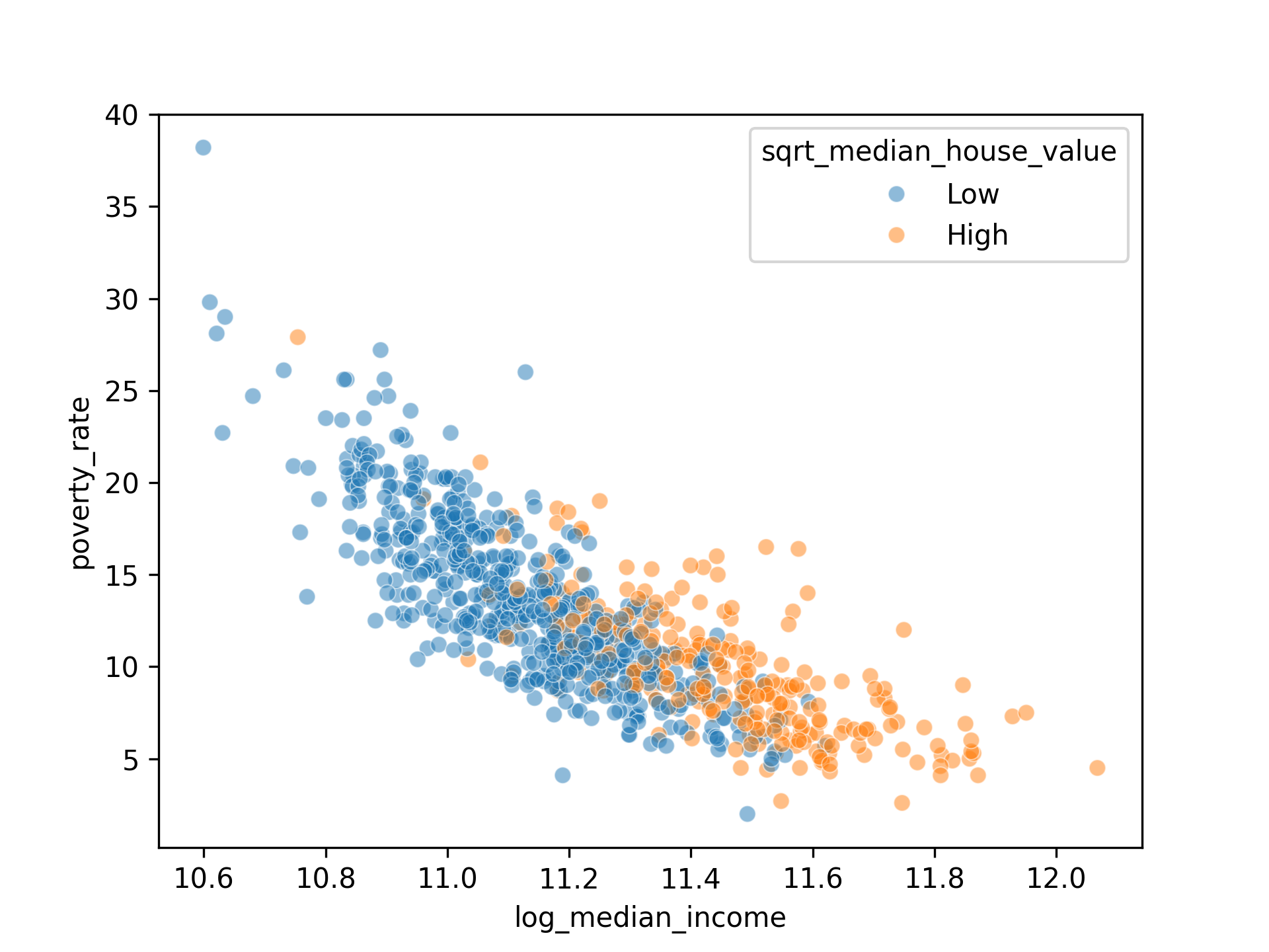
The drop in poverty rate with increasing income appears steeper for counties with lower house value (blue cluster) than ones with higher house value (orange cluster). This means that the effect of income on poverty varies depending on house values.
Here’s the interaction term:
df2['income_x_house_value'] = (df2['log_median_income'] * df2['sqrt_median_house_value'])
- Finally, robust standard errors (HC3) were used to produce more reliable p-values in the presence of heteroscedasticity.
Once I transformed the response variable and introduced interaction, I get a clearer, more interpretable model.
👉 See my notebook for application of analytical methods.
Project Outcomes
Model’s Predictive Power and Significance
The refined model was statistically significant and explained over 83% of the variation in poverty on unseen data.
My refined regression model worked well and explained 79.6% of the variance in poverty rates in training data and 83.1% in the test set. That’s high, especially for social data, where perfect predictions are rare.
Since the p-value is well below 0.05, we reject the null hypothesis. This indicates the model as a whole is statistically significant.
Final model summary:
                            OLS Regression Results
==============================================================================
Dep. Variable:      sqrt_poverty_rate   R-squared:                       0.796
Model:                            OLS   Adj. R-squared:                  0.793
Method:                 Least Squares   F-statistic:                     312.2
Date:                Wed, 04 Jun 2025   Prob (F-statistic):          2.10e-219
Time:                        00:29:01   Log-Likelihood:                -139.94
No. Observations:                 674   AIC:                             297.9
Df Residuals:                     665   BIC:                             338.5
Df Model:                           8
Covariance Type:                  HC3

Notes:
[1] Standard Errors are heteroscedasticity robust (HC3)
R-squared (test set): 0.8310581036269753
Mean Squared Error: 0.07192225315999502
Model’s Validity
Overall, the final model met the linear regression assumptions and its results (coefficients, p-values) can be trusted for inference.
Residual vs fitted plot: Was used to evaluate model fit and assumption validity, such as linearity and homoscedasticity.
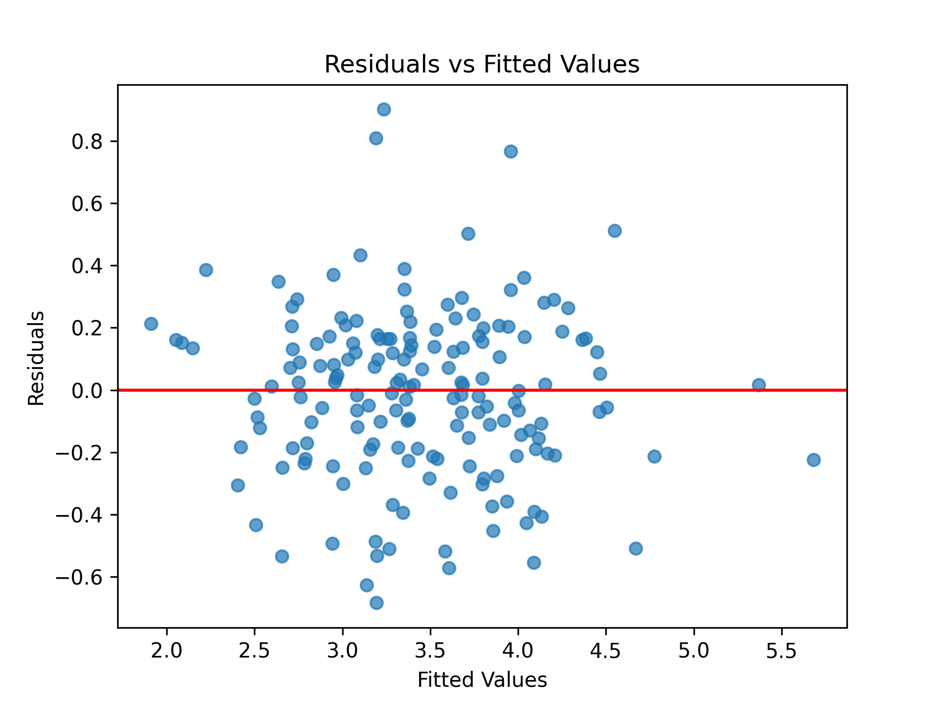
Residuals are randomly scattered around zero with consistent spread across fitted values. This means there is no major heteroscedasticity. A few mild outliers are present.
Residuals vs predictors plots: Were used to detect potential non-linear relationships or predictors that could benefit from transformations.
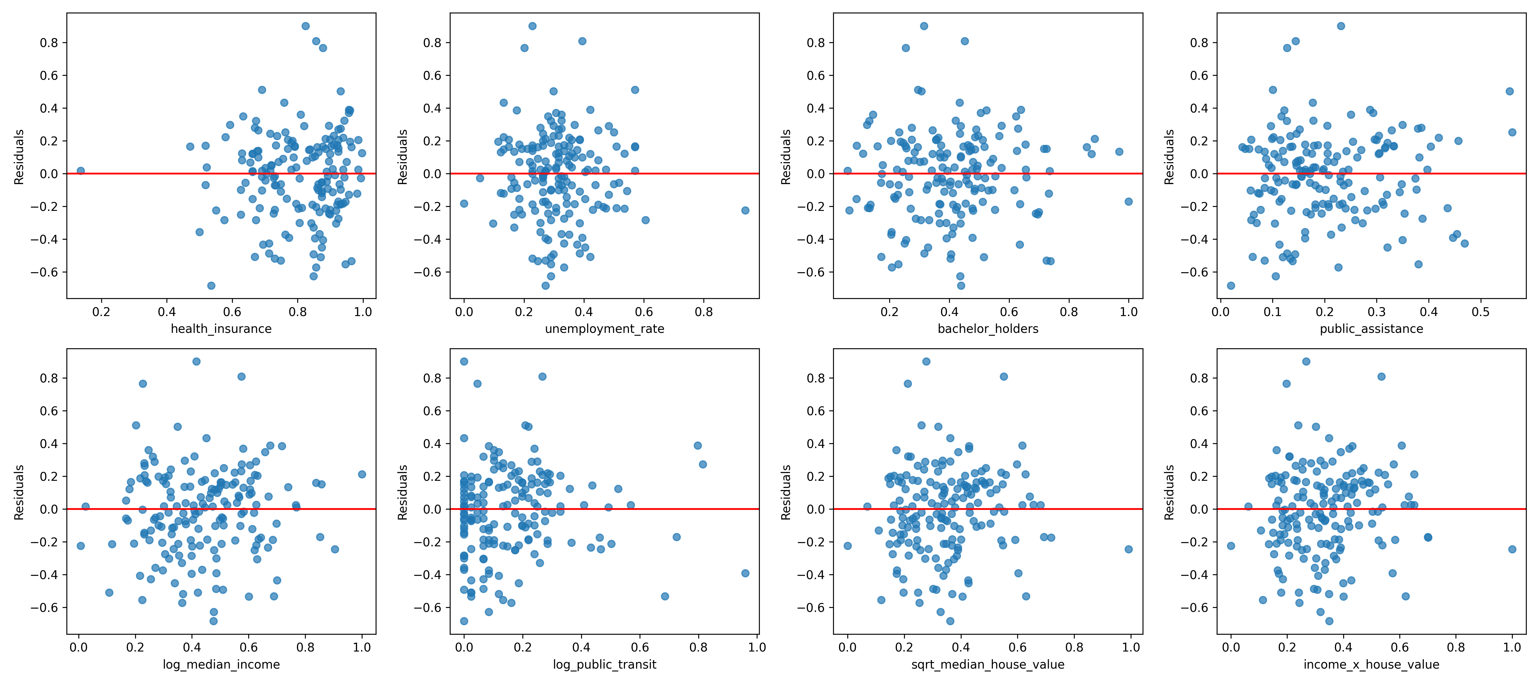
No strong patterns or funnel shapes. This supports the assumption of constant variance and linearity across predictors.
Histogram and boxplot: Were used to assess whether residuals are normally distributed.
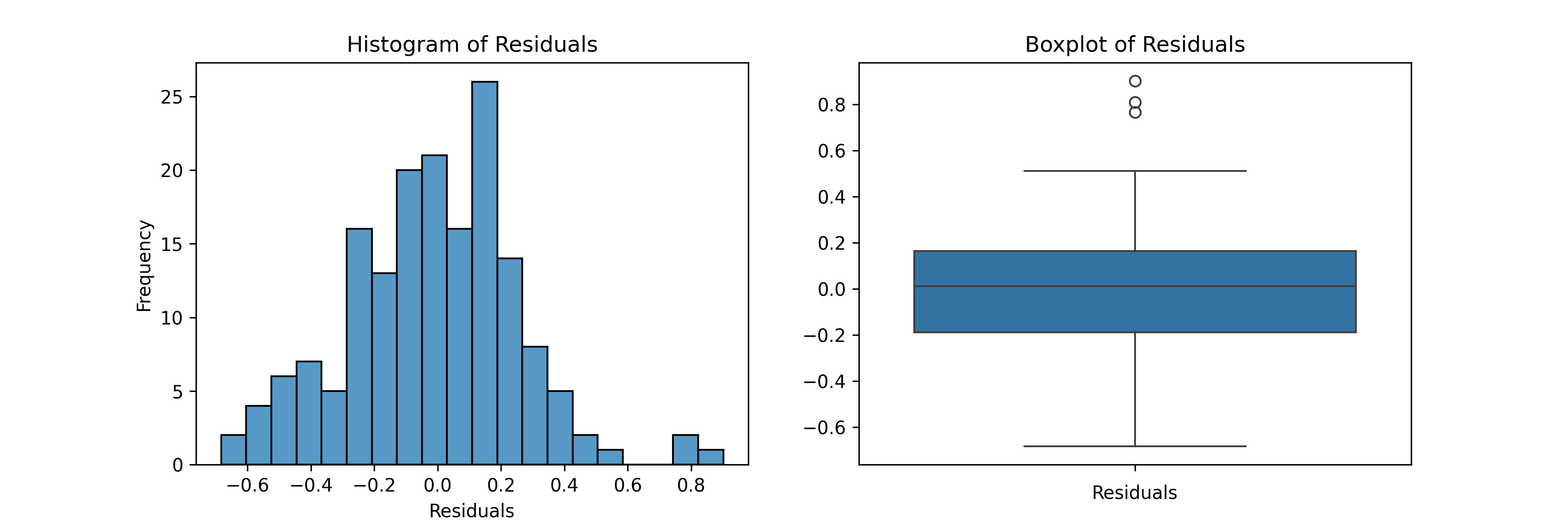
- Histogram and boxplot of residuals: Distribution is roughly normal, bell-shaped, and symmetrical. The median is near zero, with a few mild upper-end outliers.
Q-Q plot: Was used to assess normality of residuals by comparing their distribution to a theoretical normal distribution.
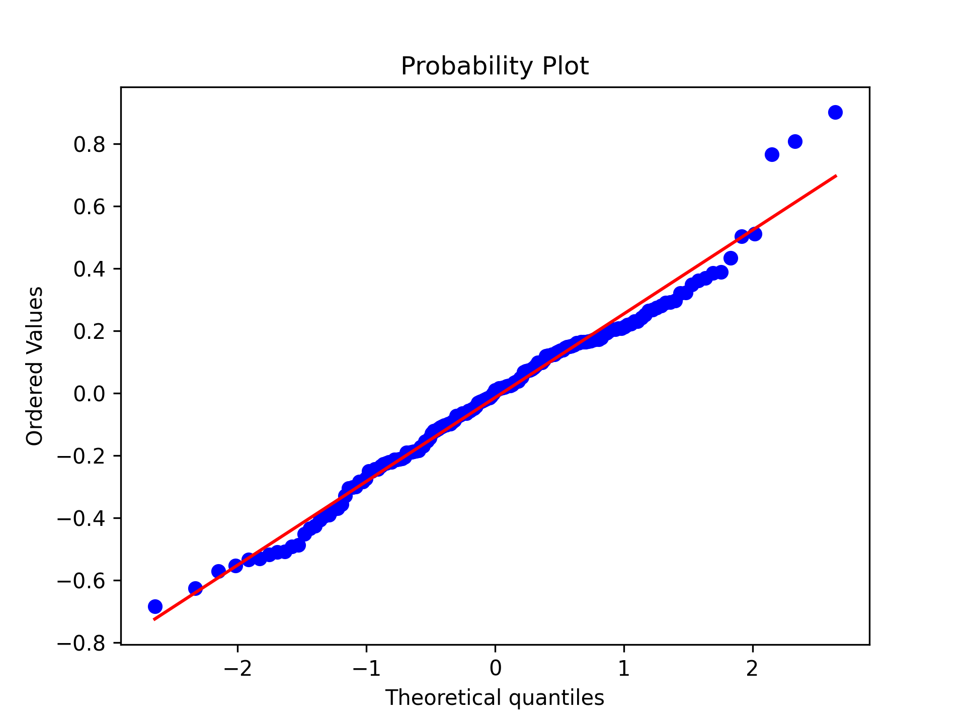
- Q-Q plot: Residuals closely follow the normal line with a slight deviation in the upper tail, which is acceptable.
Most Impactful Predictors
Statistical Significance of Individual Predictors
Public assistance may still matter, despite not being statistically significant, due to how poverty is defined.
===========================================================================================
                              coef    std err          z      P>|z|      [0.025      0.975]
-------------------------------------------------------------------------------------------
const                       5.0828      0.125     40.570      0.000       4.837       5.328
health_insurance           -0.3674      0.107     -3.445      0.001      -0.576      -0.158
unemployment_rate           0.8111      0.109      7.411      0.000       0.597       1.026
bachelor_holders            0.1332      0.116      1.149      0.251      -0.094       0.360
public_assistance           0.0735      0.120      0.613      0.540      -0.162       0.309
log_median_income          -5.2078      0.252    -20.651      0.000      -5.702      -4.713
log_public_transit          0.7545      0.095      7.940      0.000       0.568       0.941
sqrt_median_house_value   -18.3796      3.244     -5.666      0.000     -24.738     -12.021
income_x_house_value       20.4523      3.399      6.018      0.000      13.791      27.113
Based on the predictors’ p-values in the model’s summary above:
- Significant predictors included median income, median house value, health insurance coverage, public transit use, and an income × house value interaction.
- Surprisingly, public assistance rates and the percentage of bachelor’s degree holders were not statistically significant in the final model. This means that these factors have limited unique contribution to predictive power of the model once other variables were controlled.
It is important to note that unlike SPM, the OPM does not include non-cash public assistance (like SNAP, housing subsidies, TANF) in its calculation. So counties with high assistance rates may not show reduced poverty under OPM even though aid might be helping in reality.
Relative Importance of Individual Predictors
Counties with higher home values and incomes tend to have lower poverty rates, but each factor’s impact weakens as the other increases.
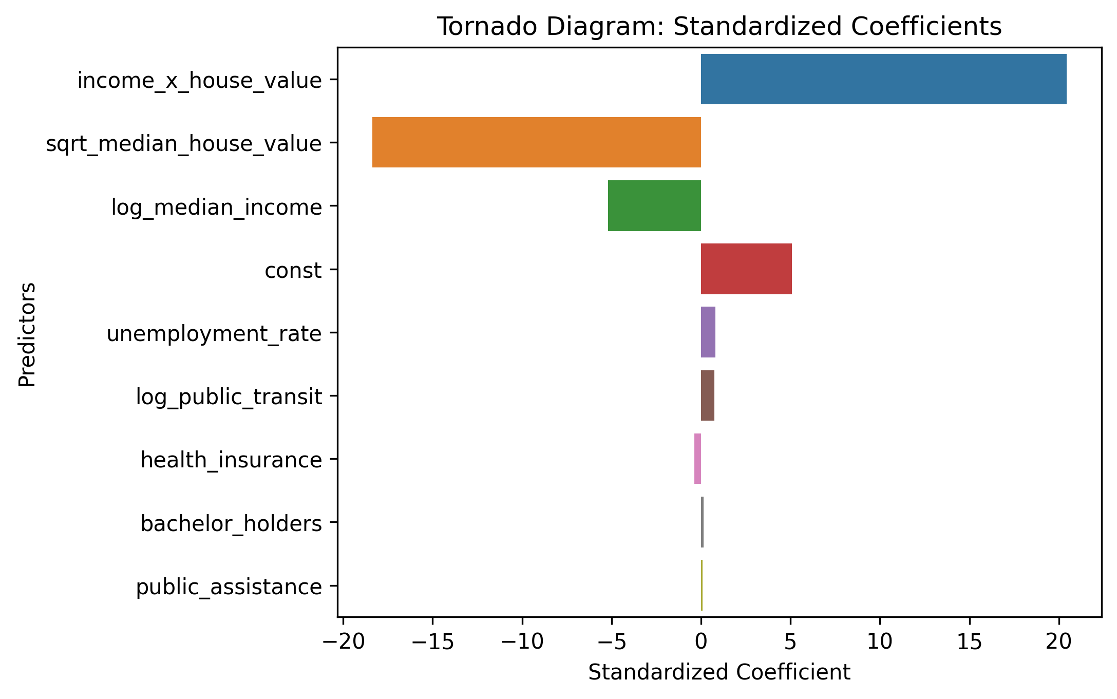
- The interaction between income and house value had the largest impact. A positive coefficient for the interaction term suggests that as income increases, the negative effect of house value on poverty becomes less strong, or as house value increases, the negative effect of income on poverty rate weakens.
- The most impactful predictors of poverty rates are median house value and median household income as they both show strong negative relationships. Counties with higher home values and incomes tend to have lower poverty rates.
- Other variables had smaller coefficients but still measurable effects.
- Higher unemployment associates with higher poverty
- Greater health insurance coverage comes with lower poverty
- More public transit use relates to higher poverty (possibly reflecting urban conditions)
- Another interesting finding is that median household income in the base model had a positive coefficient (4.7) (see the base model summary), which was unexpected because a regression plot between poverty rate and median household income suggests otherwise. However, in the refined model, the sign of this coefficient flipped due to the interaction term (see predictors’ metrics). The negative coefficient means that higher housing values are associated with lower poverty rates. This adjusted effect of median house values in the final model aligns more with general economic assumptions.
Recommended Courses of Action
A local government or policymaker could use this model to identify counties most at risk based on these factors and effectively target resources or policies.
- Invest in income growth and housing affordability: These were the strongest predictors of lower poverty. Policies targeting wage growth, job access, and affordable housing could significantly reduce poverty rates.
- Expand access to health insurance: Health insurance coverage was significantly linked to lower poverty. Improving coverage could reduce financial hardship and support poverty reduction efforts.
Final Thoughts
This project demonstrates how careful data wrangling, transparent statistical methods, and principled diagnostics can produce models that are both insightful and trustworthy. It also highlights the importance of questioning assumptions, especially when working with policy-related data.
Not every result was expected. Public assistance didn’t come through as a statistically significant predictor likely due to limitations of the Official Poverty Measure (OPM), which does not account for non-cash assistance like SNAP or housing vouchers. That’s a flaw in the poverty definition itself, not necessarily in the data.
This is a reminder: statistics model relative relationships, not realities. The real world is messier. Numbers can’t fully capture dignity, barriers, or the trade-offs that people in poverty navigate every day. Still, we can quantify strong patterns, and we should, especially when it helps guide policymakers, public agencies, and community organizations in prioritizing resources and interventions.
If you’re a policymaker, nonprofit leader, or fellow data scientist: I hope this analysis adds value to your work or sparks new questions worth pursuing.
References
- Creamer, J., & King, M. D. (2024, November 14). How Do Policies and Expenses Affect Supplemental Poverty Rates?